A Tutorial on Analyzing and Interpreting Movies
Authors: Akshay Anil, Atul Bharati, Chaewoon Hong
Welcome to our tutorial on how to analyze data on movies! This dataset was pulled from a movies database and is available on Kaggle, courtesy of The Movie Database (TMDb). It contains information on 5000 popular movies. By analyzing the dataset, we may be able to find the magic formula needed for movies to become successful. We will be looking to see if genre and budget are key factors by having a null hypothesis of no correlation between the three.
In this tutorial, we will be walking you step by step in how to approach this dataset in order to get the data you want. We will be analyzing the data we collect with the help of visual graphics.
Our code is written in Python 3 on the Jupyter Notebook.
We start off by importing all the libraries that we will need in this project:
- pandas - used to store our dataset in a table
- numpy - provides mathematical functions to help us analyze the data
- matplotlib - allows us to graph our data
- warnings - suppresses any warnings we run into
- re - used for regular expressions
- cpi - we will be using the inflation method to account for money value over time
- datetime - used in conjunction with economics
- sklearn - library for machine learning
- statsmodels - used to verify our null hypothesis
If you happen to get an error like this:
No module named 'module_name'
Simply go to the terminal and run
pip install module_name
import pandas as pd
import numpy as np
import matplotlib.pyplot as plt
import seaborn as sns
import warnings
import re
import cpi
import datetime
from sklearn import linear_model
from statsmodels.formula.api import ols
warnings.filterwarnings('ignore')
For this tutorial, we downloaded the dataset from Kaggle and saved it as movie_list.csv. Even though CSV stands for Comma-Separated Values, we need to confirm that other characters such as semi-colons are not used instead. We do this by opening the file with a text editor and searching for delimiters.
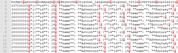
Here we see that commas are used, so we add sep=',' as an argument to the read_csv function.
Let's take a look at the dataset that we have.
# Display the data as is from the source
movies = pd.read_csv('movie_list.csv', sep=',')

# Display the first five rows
movies.head()
We get a table with 20 columns! Let's trim down the dataset so we are left with movies that are originally in English and have already been released. We also want to remove any rows where the revenue or budget is equal to 0.
# Limit movies to those that are in English and already Released for a fair comparison
movies = movies[movies.original_language == 'en']
movies = movies[movies.status == 'Released']
# We want movies that at least had a budget and had a revenue
movies = movies[movies.budget >= 0]
movies = movies[movies.revenue >= 0]
# Remove movies that are not categorized into genres
movies = movies[movies.genres != '[]']

# Remove columns that are not vital for analysis
movies.drop(columns=['popularity', 'original_language', 'status', 'keywords', 'original_title', 'overview', 'homepage', 'id', 'production_companies', 'production_countries', 'spoken_languages', 'tagline'], inplace=True)

# Remove any rows with missing data
movies.dropna(inplace=True)
Let's create some functions to split up the release date so we can analyze changes over months, days, and years.
# Functions to split up release_date
def get_year(row):
    date = row['release_date']
    y, _, _ = date.split("-")
    return int(y)
def get_month(row):
    date = row['release_date']
    _, m, _ = date.split("-")
    return int(m)
def get_day(row):
    date = row['release_date']
    _, _, d = date.split("-")
    return int(d)
# Create and set year, month, and day of release for each movie
movies['release_year'] = movies.apply(get_year, axis=1)
movies['release_month'] = movies.apply(get_month, axis=1)
movies['release_day'] = movies.apply(get_day, axis=1)

# Remove the release_date column because we don't need it anymore
movies.drop(columns=['release_date'], inplace=True)
movies.head()
The value of a dollar changes over time so we should take that into consideration. Below we create two methods, one for budget and one for revenue, to update their values to what they are worth in 2018.
def get_current_budget(row):
    return cpi.inflate(int(row['budget']), datetime.date(row['release_year'], row['release_month'], row['release_day']),
datetime.date(2018,1,1))

def get_current_revenue(row):
    return cpi.inflate(int(row['revenue']), datetime.date(row['release_year'], row['release_month'], row['release_day']),
datetime.date(2018,1,1))
# Replace existing budget and revenue values with those adjusted for inflation
movies['budget'] = movies.apply(get_current_budget, axis=1)
movies['revenue'] = movies.apply(get_current_revenue, axis=1)

movies.head()
Now let's swap some columns to make the dataframe easier to read.
# Swap the headers
# Budget with title
col_list = list(movies)
col_list[0], col_list[5] = col_list[5], col_list[0]
# budget with popularity
col_list[2], col_list[5] = col_list[5], col_list[2]

# Swap the values of the columns
movies.columns = col_list
c = movies.columns
# Budget with title
movies[[c[0], c[5]]] = movies[[c[5], c[0]]]
# Budget with popularity
movies[[c[2], c[5]]] = movies[[c[5], c[2]]]

movies.head()
Great! This looks like something we can work with. Let's run a quick dataframe describe to identify invalid data. In respect to the data we are using, none of the values should be negative (Negative runtime? What would that even look like?).
movies.describe()
Perfect! Now let's start visualizing the data we cleaned up.
Graphing
Tracking budget over the years might be interesting to see. However, not all years are equally represented in terms of number of movies. How do work around this problem? Unlike the mean, the maximum value is not impacted by the number of values. Let's try plotting maximum budget per year.
plt.figure(figsize=(25, 10));
# Gives us lines a background to help line up bars with their values
sns.set()
# Get the total budget and revenue per year
budget_year = movies.groupby(['release_year'])['budget'].max()
budget_year = pd.DataFrame({'release_year':budget_year.index, 'max_budget':budget_year.values})
# Plot the data
sns.barplot(budget_year['release_year'], budget_year['max_budget'])
plt.title('Max Budget Per Year')
plt.xlabel('Year')
plt.ylabel('Budget ($100M)')
plt.xticks(rotation=45)
plt.show()

The plot shows how the budget for movies has clearly risen over the years. This could perhaps be explained by the advancement of technology and the incorporation of high quality sets.
Looking at the Genres
Next we'll be looking at the genres of the movies and take a look at the average rating per genre. We'll be using the same movies variable because it contains all the columns that we will be needing. We'll be using regular expressions to extract the genre names from the 'genres' column.
# The format of the genres column is a string that looks like this:
# [{"id": 12, "name": "Adventure"}, {"id": 14, "name": "Fantasy"}, {"id": 28, "name": "Action"}]
# We only want the genres after "name":, so we will use regex to eliminate the other characters.

# Iterate through the rows
for index,row in movies.iterrows():
    # Initialize a new string - this will replace the row value for genre to make it easier to read and extract
    display_genres = ""
    # Isolates the name: (genre) from the ids
    g = re.findall(r"name\": \"\w+", row['genres'])
    # g should now look like this:
    # ['name": "Action', 'name": "Adventure', 'name": "Fantasy', 'name": "Science']

    # Iterate through each item in g and remove everything but the genres
    for item in g:
        remove = re.search("name\": \"", item)
        display_genres += (item[:remove.start()] + item[remove.end():]) + " "
    display_genres = display_genres[:-1]
    display_genres = display_genres.split(' ')
    # Replace the genre value with the new list
    movies.at[index, 'genres'] = display_genres
movies.head()
Having a list of genres per movie makes it difficult to analyze each genre separately. Let's unpack the list so that each row only has one genre.
# Break down the list and create a new dataframe with the split genres
movies = pd.DataFrame([(d, tup.title, tup.budget, tup.revenue, tup.runtime, tup.vote_average, tup.vote_count, tup.release_year, tup.release_month, tup.release_day) for tup in movies.itertuples() for d in tup.genres])
# Give the columns the names they used to have
movies.columns=['genre', 'title', 'budget', 'revenue', 'runtime', 'vote_average', 'vote_count', 'release_year', 'release_month', 'release_day']
movies.head()
Sweet! Avatar used to have the value [Action, Adventure, Fantasy, Science], but now they are their own rows. This is called melting.
# Get all the possible genres from the dataset
# the keys of the genres dict will have the genre names and the values will be the sum of the average ratings for that
# particular genre
genres = {}
# average_counter is a dict that will have the same keys as genres dict but its values will be the number of average ratings
average_counter = {}

for index, row in movies.iterrows():
    item = row['genre']
    if item not in genres:
        # Initialize the keys as 0/1 first
        genres[item] = 0
        genres[item] += row['vote_average']
        average_counter[item] = 1
    else:
        genres[item] += row['vote_average']
        average_counter[item] += 1

# Displayed below are all the possible genres (keys) from this dataset
genres
# Include the average ratings
average_ratings = []
for (sum, denom) in zip(genres.values(), average_counter.values()):
    if denom != 0:
        average_ratings.append(sum/denom)
    else:
        average_ratings.append(0)

# Include the number of movies
xvals = []
for (genre, count) in zip(genres.keys(), average_counter.values()):
    xvals.append(genre + " (" + str(count) + ")")

plt.figure(figsize=(25, 10))
sns.barplot(xvals, average_ratings)
plt.title('Average Voter Ratings Per Genre')
plt.xlabel('Genre')
plt.ylabel('Average Rating (1-10)')
plt.xticks(rotation=45)
plt.show()

It is quite difficult to compare each genre's ratings with the other ratings, so let's sort the histograms. We'll be doing a lot of sorting in this tutorial so let's create a function for sorting.
def sort_graph(xlist, ylist):
    # initialize to_sort as a dict. The keys will be the xlist (where order doesn't matter like genre names / movie titles)
    # and the values will be the ylist (ex. average  budget, avarege rating).
    # When we sort the ratings (values), the movie names (keys) will still remain with its rating value.
    to_sort = {}
    for (x,y) in zip(xlist,ylist):
        to_sort[y] = x

    # sort the values
    sorted_by_value = sorted(to_sort.items(), key=lambda kv: kv[1])

    xout = []
    yout = []
    for (x, y) in sorted_by_value:
        xout.append(x)
        yout.append(y)

    return xout,yout
genres,ratings = sort_graph(average_ratings,xvals)

plt.figure(figsize=(25, 10))
sns.barplot(genres, ratings)
plt.title('Average Rating Per Genre (Sorted)')
plt.xlabel('Genre')
plt.ylabel('Average Rating (1-10)')
plt.xticks(rotation=45)
plt.show()

From this graph, we can see that the horror genre seems to have the lowest average ratings compared to the other genres. The reason we put the number of movies in parenthesis next to the genre titles is that some genres have smaller samples which means the average ratings for a particular genre may not be a true representation of the population.
For example, the "Foreign" genre had only one movie with a rating of 6.9. Even if the Foreign genre only has one movie, if it was plotted on the graph, it would seem like the Foreign genre has the highest average rating out of all other genres. For this very reason, we removed the Foreign genre from the graph and put the number of movies in parenthesis as a precaution.
Taking a Closer Look
Now that we have cleaned up the genres column, let's take a closer look into the Horror genre. Compared to the other genres, the Horror genre has a significantly lower average rating than the other genres. First, let's plot the horror movies individually to see their ratings.
horror_title = []
horror_rating = []
for index, row in movies.iterrows():
    if row['genre'] == 'Horror':
        horror_title.append(row['title'])
        horror_rating.append(row['vote_average'])

titles,ratings = sort_graph(horror_rating,horror_title)

plt.figure(figsize=(30, 12))
sns.barplot(titles, ratings)
plt.title('Average Voter Ratings For Horror Movies')
plt.xlabel('Movie Title')
plt.ylabel('Average Rating (1-10)')
plt.xticks(rotation=90)
plt.xticks(np.arange(0,len(horror_title),3))
plt.show()
print("(Every 3rd Movie Label is labelled for ease of read)")

Perhaps the reason the horror movies have lower ratings than all other genres is because of the budgets. Let's look at the average budget for each genre to see if it plays a role in the low ratings. We'll use code that is very similar to the one we used previously to find the average ratings.
genre_budget = movies.groupby(['genre'])['budget'].mean()
genre_budget = pd.DataFrame({'genre':genre_budget.index, 'average_budget':genre_budget.values})
# the keys of the dict will have the genre names and the values will be the sum of the budgets for that particular genre
genres = {}
# average_counter is a dict that will have the same keys as genres but its values will be the number of values
average_counter = {}

for index, row in movies.iterrows():
    item = row['genre']
    if item not in genres:
        # Initialize the keys as 0/1 first
        genres[item] = 0
        genres[item] += row['budget']
        average_counter[item] = 1
    else:
        genres[item] += row['budget']
        average_counter[item] += 1

# Include the average budgets
average_budget = []
for (sum, denom) in zip(genres.values(), average_counter.values()):
    if denom != 0:
        average_budget.append(sum/denom)
    else:
        average_budget.append(0)

# Include the number of movies
xvals = []
for (genre, count) in zip(genres.keys(), average_counter.values()):
    xvals.append(genre + " (" + str(count) + ")")

plt.figure(figsize=(20, 10))
sns.barplot(xvals, average_budget)
plt.title('Average Budget Per Genre')
plt.xlabel('Genre')
plt.ylabel('Average Budget ($100M)')
plt.xticks(rotation=45)
plt.show()

Since the values in the x-axis (genres) don't have a particular order, let's reorder the genres so we can easily look at how the genres are related to each other when it comes to average budget.
genres,budgets = sort_graph(average_budget,xvals)

plt.figure(figsize=(20, 10))
sns.barplot(genres, budgets)
plt.title('Average Budget Per Genre (Sorted)')
plt.xlabel('Genre')
plt.ylabel('Average Budget ($100M)')
plt.xticks(rotation=45)
plt.show()

Again, the horror genre is near last when it comes to its budget. Now let's see the relationship between the average rating and average budget for each genre.
plt.figure(figsize=(15, 10))
plt.scatter(average_budget, average_ratings)
plt.title('Relationship Between Budget and Ratings for Every Genre')
plt.xlabel('Budget')
plt.ylabel('Rating')

for i in range(len(average_budget)):
    plt.text(average_budget[i], average_ratings[i], xvals[i], fontsize=12)

# Draw the regression line
# m = slope, b = y-intercept
m, b = np.polyfit(average_budget, average_ratings, 1)

# Calculate y=mx+b for each point and then create regression line
yvals = []
index = 0
for y in average_ratings:
    yvals.append(m*average_budget[index]+b)
    index += 1
plt.plot(average_budget, yvals , 'r')
plt.show()

Looking at the regression line, although for the horror genre it seems that budget and rating go hand in hand, the line is more horizontal than vertical but has a slightly negative slope. This implies that there's actually not much of a correlation, or relationship, between the budget of a film and the average voter rating.
Linear Regression Modelling (Machine Learning)
We can use a machine learning algorithm like linear regression to make a model and predict the dependent/response variable given a value for the independent/explanatory variable. To learn more about the basics of linear regression, visit this link.
In this example, we will try to predict the revenue of action movies given the budget of action movies. This is an example of simple linear regression since there's only one independent (x-axis) variable involved.
action_movies = movies[movies.genre == 'Action']
action_movies.head()
plt.figure(figsize=(15, 10))
plt.scatter(action_movies['budget'], action_movies['revenue'])
plt.title('Budget vs Revenue for Action Movies')
plt.xlabel('Budget (per $100M)')
plt.ylabel('Revenue (per $1B)')

reg = linear_model.LinearRegression()
X = [[budget] for budget in action_movies['budget'].values]
y = [[revenue] for revenue in action_movies['revenue'].values]
reg_model = reg.fit(X, y)

plt.plot(X, reg_model.predict(X))

Even though most of the data points are clustered near the bottom left, meaning that the budget and revenue for those action movies are relatively low, the regression line model indicates that there's some positive association between budget and revenue.
The line of code below shows how we can use this linear regression model:
print(reg_model.predict([[150000000]]))
The value inside the square brackets is the input value (in this case, the budget) and the predict function will determine the output (the revenue) based on the regression line depicted above. The revenue for an action movie will be about 450 million dollars if a movie crew has 150 million dollars to spend to create the movie.
The value below gives the slope of the regression line:
reg_model.coef_
It indicates that there's about 3 dollars in revenue for every dollar in budget for action movies.
Now let's see if we can fit a linear regression model for revenue including a term for an interaction between budget and genre. More information about interaction terms can be found here.
arr = []
# assigns an index to each genre
for index, row in movies.iterrows():
    if 'Action' in row['genre']:
        arr.append(0)
    elif 'Documentary' in row['genre']:
        arr.append(1)
    elif 'Horror' in row['genre']:
        arr.append(2)
    elif 'Music' in row['genre']:
        arr.append(3)
    elif 'Romance' in row['genre']:
        arr.append(4)
    elif 'Drama' in row['genre']:
        arr.append(5)
    elif 'Crime' in row['genre']:
        arr.append(6)
    elif 'Comedy' in row['genre']:
        arr.append(7)
    elif 'Mystery' in row['genre']:
        arr.append(8)
    elif 'Thriller' in row['genre']:
        arr.append(9)
    elif 'Western' in row['genre']:
        arr.append(10)
    elif 'History' in row['genre']:
        arr.append(11)
    elif 'War' in row['genre']:
        arr.append(12)
    elif 'Science' in row['genre']:
        arr.append(13)
    elif 'Action' in row['genre']:
        arr.append(14)
    elif 'Family' in row['genre']:
        arr.append(15)
    elif 'Fantasy' in row['genre']:
        arr.append(16)
    elif 'Adventure' in row['genre']:
        arr.append(17)
    elif 'Animation' in row['genre']:
        arr.append(18)
    elif 'Foreign' in row['genre']:
        arr.append(19)
    elif 'TV' in row['genre']:
        arr.append(20)

movies['genre_index'] = pd.Series(data=arr, index=movies.index)
# Fit a model for revenue including a term for an interaction between budget and genre
reg_model = ols(formula="revenue ~ budget*genre_index", data=movies).fit()
# displays linear regression model data
reg_model.summary()
The table above gives the ordinary least squares (OLS) regression results. We will direct our attention to the second portion of the table, which contains the p-values for each variable. Feel free to look at this guide to assist you with the understanding of regression table results.
The p-value column (P>|t|) gives probabilities that can help you determine whether or not the null hypothesis should be rejected: the coefficient is equal to 0, which indicates no effect. A low p-value (< 0.05) indicates that the null hypothesis should be rejected, meaning that changes in independent variable relate to those in the dependent variable. Otherwise, if the p-value is high (>= 0.05), then the variable might not be a good fit for the model. In our example, this isn't a problem for for budget and genre because their p-values are both below 0.05. However, our null hypothesis that the combination of budget and genre is a bad indicator for revenue is proven slightly correct with a p-value of 0.077 that is slightly over 0.05.
The other main column of interest is coefficient. We'll specifically use the budget variable in the analysis. The value of the coefficient is given as 2.7063 which indicates that for every additional dollar spent for the budget, we expect about 2 dollars and 71 cents increase in revenue/profits. This is simply the slope of the regression line for this model that was created.
Conclusion
As it can be seen, taking a dataset and playing around with it can be intriguing and you can learn many things if you try analyzing it like to the extent we did.
After we set up the dataframe properly by modifying the columns and some values in some cells like in the genres column, we were able to perform analysis on the bar graphs and scatter plots we created. For example, we looked at the average voter ratings per genre and after sorting the bars in an ascending order, we realized that horror movies tend to have the lowest ratings. Then, we delved in deeper by analyzing the average voter ratings for all the individual horror movies in the dataset and realized that most of the ratings were relatively low, thus proving why horror movies have low ratings in general. In terms of budgets for creating movies, horror movies were near the bottom of all the movie categories so there's a possible relationship between voter ratings and budgets of various movies. We performed linear regression between those two variables and realized that there's a slight positive correlation.
For the machine learning aspect of this tutorial, we focused on the budget and revenue of action movies by creating a simple linear regression model. We realized that there was some positive association between the budget and revenue based on the scatter plot and OLS regression results table. The regression model can be used to predict the revenue/profits (in billions of dollars) of an action movie based on the expenditures (in terms of hundreds of millions of dollars) for creating the movie, which is nice for extrapolation or predicting outside the range of the given x values.
We hope you have taken something of value and use from this tutorial!